Robust Optimization
A simple portfolio example (Bertsimas and Sim 2004) is utilized to demonstrate how to define random variables and uncertainty sets in XProg. Suppose that there are \(n=150\) stocks to be selected, and the uncertain return of each stock \(i\), denoted by \(\tilde{p}_i\), is within a symmetric interval \(\left[p_i-\sigma_i, p_i+\sigma_i\right]\), where \(p_i\) is the expected return, and \(\sigma_i\) is a measure of uncertainty for stock \(i\). The uncertainty set \(\mathcal{Z}\) is formulated as the following equation.
\begin{align}
\mathcal{Z}=\left\{\pmb{z}:~\|\pmb{z}\|_{\infty}\leq 1, \|\pmb{z}\|_1\leq \Gamma\right\}
\end{align} The robust optimization model for this portfolio problem can be expressed as the problem below.
\begin{align}
\min~&\max\limits_{\pmb{z}\in\mathcal{Z}} \sum\limits_{i=1}^n\left(p_i+\sigma_iz_i\right)x_i \\
\text{s.t.}~&\sum\limits_{i=1}^nx_i=1\\
&\pmb{x}\geq \pmb{0}
\end{align} In this example, it is assumed that the budget of uncertainty \(\Gamma=5\), and the values of each \(p_i\) and \(\sigma_i\) are given as the following equations.
\begin{align}
&p_i=1.15+i\frac{0.05}{150} \\
&\sigma_i=\frac{0.05}{450}\sqrt{2n(n+1)i}
\end{align} These two equations imply that the stock with higher expected returns also have higher levels of uncertainty. This robust optimization model can be simply represented by the code listed below.
n  = 150;                                % number of stocks
p  = 1.15+ 0.05/150*(1:n)';              % mean return
sigma = 0.05/450*sqrt(2*n*(n+1)*(1:n)'); % deviation
Gamma = 5;

model=xprog('portfolio');                % create a model, named "portfolio"

x=model.decision(n);                     % decisions as fraction of investment, an n*1 vector

% random variables and the uncertainty set
z=model.random(n);                       % random deviations from the expected returns, as an n*1 vector
u=model.random(n);                       % the absolute values of z, as an n*1 vector
model.uncertain(abs(z)<=1);              % norm_inf(z)<=1
model.uncertain(abs(z)<=u);              % expressing the absolute value of z
model.uncertain(sum(u)<=Gamma);          % norm(z)<=Gamma

r = p + sigma.*z;                        % random return of stocks
model.max(r'*x)                          % define objective
model.add(sum(x)==1);                    % constraint of x
model.add(x>=0);                         % bound of x

model.solve;                             % solve the problem
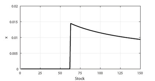
The objective value is 1.1709, and the optimal solution in terms of the percentage of resources invested in each stoch is presented by the figure below.
This case shows the steps of solving robust optimization problems by using XProg. The constraints of random variables can be included into the uncertainty set by function "uncertain". Note that users must define a specific uncertainty set before solving the model, otherwise the program will be terminated with an error message.
